

Overview
In our earlier blog post on supporting full text search in SmithDB, we went over how we designed our object-storage backed inverted index implementation. In this blog post, we will cover how we construct, compact, and query this index in SmithDB.
Inverted index construction and merging
Index construction happens inline during ingestion. New runs become searchable within seconds, and because the freshest data is still resident on the node that wrote it, leading-edge queries read both the indexes and core data files directly from local storage instead of paying a round trip through object storage. On compaction, we merge indexes associated with different data files.
Payload parsing
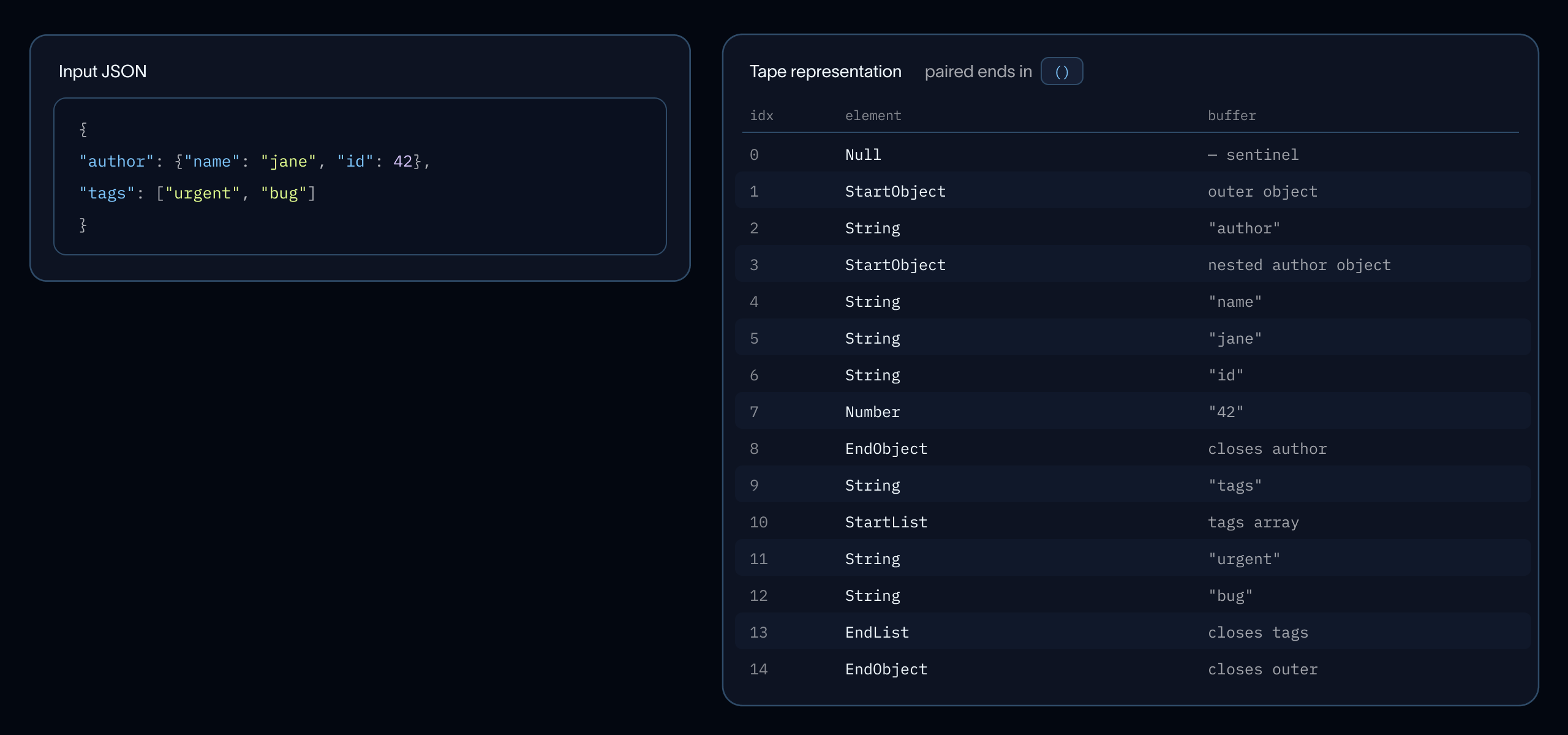
Recall that SmithDB indexes the large inputs and outputs fields (among a few others) present in run payloads. For deeply nested and large payloads, JSON parsing dominates construction time. We only need flattened key paths and leaf values, so we built a JSON tape adapted from Apache Arrow's arrow-json crate, which is itself inspired by simdjson's tape format.
Our implementation consists of a flat sequential array of tokens with all string bytes in one contiguous buffer: no per-field allocation, no numeric conversion. A single-pass iterator then flattens each document into (path, leaf_value) pairs: nested objects become dotted paths, array elements collapse onto their parent key: {"agent": "deep agents", "tags": ["langchain", "engine"]} yields (agent, "deep agents"), (tags, "langchain"), (tags, "engine").
See below for another example.
Tokenization
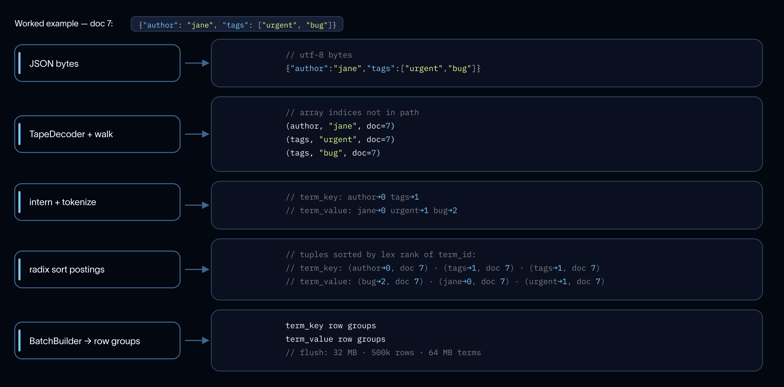
Before a value becomes an index term, it is tokenized: split on non-alphanumeric boundaries, lowercased, dropped of stop words, and capped at 256 characters.
Sorting and interning
Recall that we use finite state transducers (FSTs) for our term layout in our inverted index implementation. The flat postings table must be sorted by term before it can feed the FST writer.
Across agent traces, the same JSON paths and token values repeat in virtually every document for a particular tenant and tracing project. When implemented naively, this sort is dominated by string comparisons. To get around this, we leverage string interning: a technique that maps each unique term to a compact integer ID upfront. As a result, comparison cost scales with distinct terms, not occurrences, cutting construction time by ~2.2× in our benchmark.
We use ahash for hashing (stdlib ~20% slower, Tantivy's MurmurHash2 ~30% slower), store all bytes in one contiguous buffer, and use Hashbrown's raw API to hash each string exactly once per intern call. Each occurrence is then recorded as a (doc_id, term_rank, position) triple in a flat table. We leverage radix sort to group postings by term in O(n) before the sorted run feeds the FST writer.
Flush thresholds
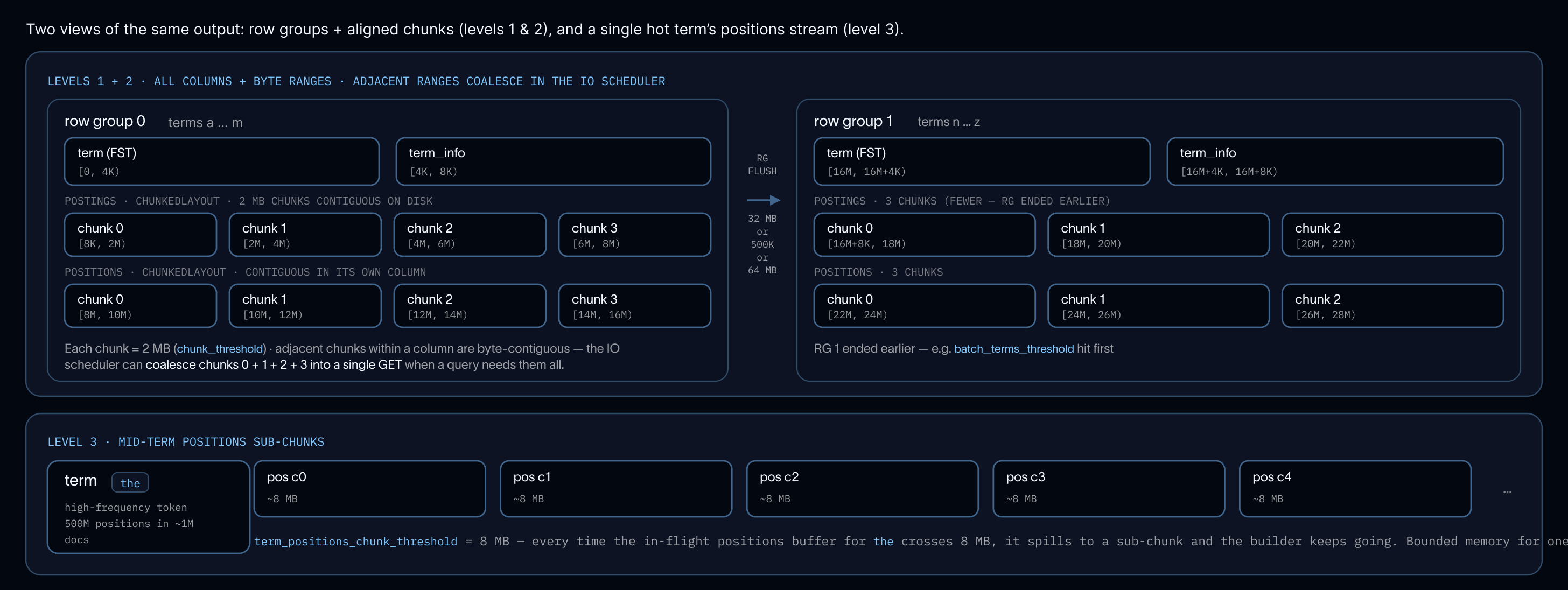
Accumulating an entire batch before writing would let a single high-frequency term (5, agent, or a common JSON key) grow unboundedly. During index write, we have optimized flush boundaries on three thresholds:
- a row group: 32 MB postings / 500 K terms / 64 MB raw term bytes, sized to keep the in-memory FST writer within addressable memory
- an aligned chunk: ~2 MB, postings and positions flush at matching document boundaries so a query reading both gets contiguous byte ranges in a single GET
- a mid-term position spill: 8 MB, an escape hatch for Zipfian tail terms like
5that would otherwise accumulate hundreds of millions of positions before the term finishes
Chunks within each column are byte-contiguous on disk, so every threshold maps directly to a worst-case GET size and a worst-case memory footprint.
Index merge
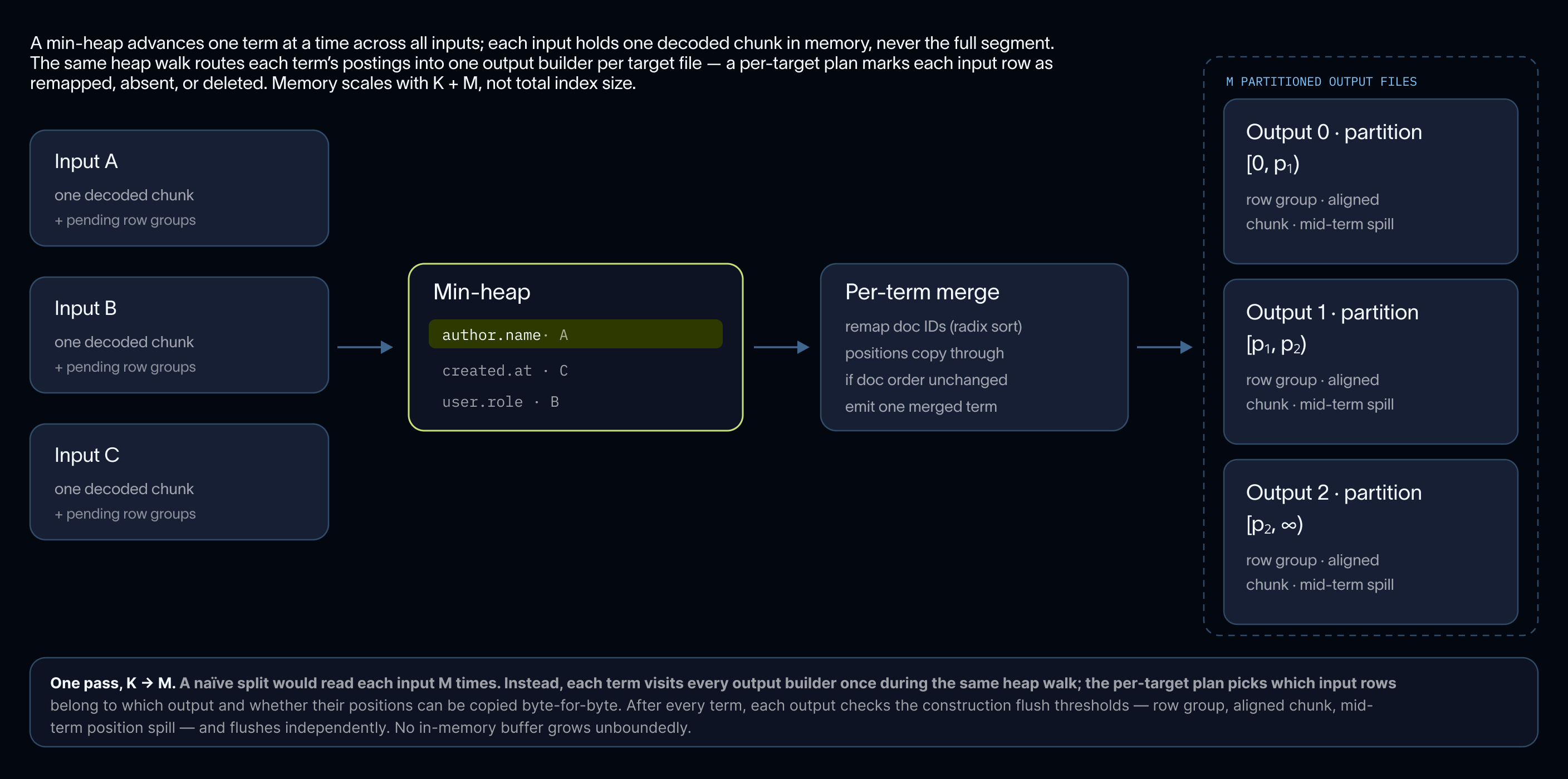
Our compaction service merges smaller files written by ingestion into larger files more optimal for querying. Along with compacting core files, the service processes each core file’s per-file indexes with a streaming merge.
A min-heap advances one term at a time across all inputs; each input holds only one decoded chunk in memory at a time, never the full segment. The merged terms emerge already sorted (required by FST writing) and the same three flush thresholds from construction (row group, aligned chunk, mid-term position spill) bound the output builder after every term. Memory scales with the number of inputs being merged, not the total index size, regardless of how many segments are involved.
Query time
The read path reuses the same machinery the rest of SmithDB queries already flow through (DataFusion and Vortex's LayoutReader pipeline) and slots the inverted index in as another layout that the planner pushes predicates into. Nothing about the SQL surface or the query planner had to learn that an index exists: it’s all handled internally by our TableProvider and LayoutReader implementations.
For a given query, after resolving the candidate segments from our metastore, the planner checks which of those segments actually have an index built for the column being queried. Segments missing an index for the queried column are quietly routed to a column scan instead; segments with an index are routed to the index. All of this happens before any object-storage request.
One segment, many files
In SmithDB, each metastore entry points to one core file holding the row data, plus a sibling file per indexed column. The challenge at query time is making this collection of files behave like a single addressable entity (both to DataFusion above and to the IO scheduler below) while still letting each predicate pick which files it actually needs to open (not all predicates require downloading and opening index files).
At plan time, each predicate is inspected once per segment and routed to one of three outcomes: read it through the index (the column is indexed in this segment), fall back to a column scan on the core file (no index available), or short-circuit to "no matches" (the column isn't projected at all). All three decisions are made before any object-storage request, so a segment with no index for the queried column never opens an index file, and a segment with one never opens the column for that predicate.
At runtime, the core file and each index file compose into a single virtual layout. DataFusion sees one logical file segment: projection pushdown, predicate pushdown, and the segment's row-index space all work uniformly across core and index columns. The IO scheduler, on the other hand, sees the actual byte ranges from each underlying file, so reads inside the same file coalesce naturally where they're adjacent and stay correctly partitioned where they aren't.
A query that touches three columns out of a hundred opens exactly three index files. A predicate that doesn't use the index never opens an index file at all. A segment that's missing an index for one column transparently falls back to a scan for just that column, without disabling indexing for the rest of the query.
The SmithDB SQL surface (json_key, json_key_search, search) is rewritten by the planner into a Vortex expression; time bounds, projections, and joins to the core file all run through unchanged DataFusion plans. The v1→v2 layout migration we described in our earlier blog post required zero changes above the Vortex layer: same expression interface, different bytes underneath.
From layout to GETs
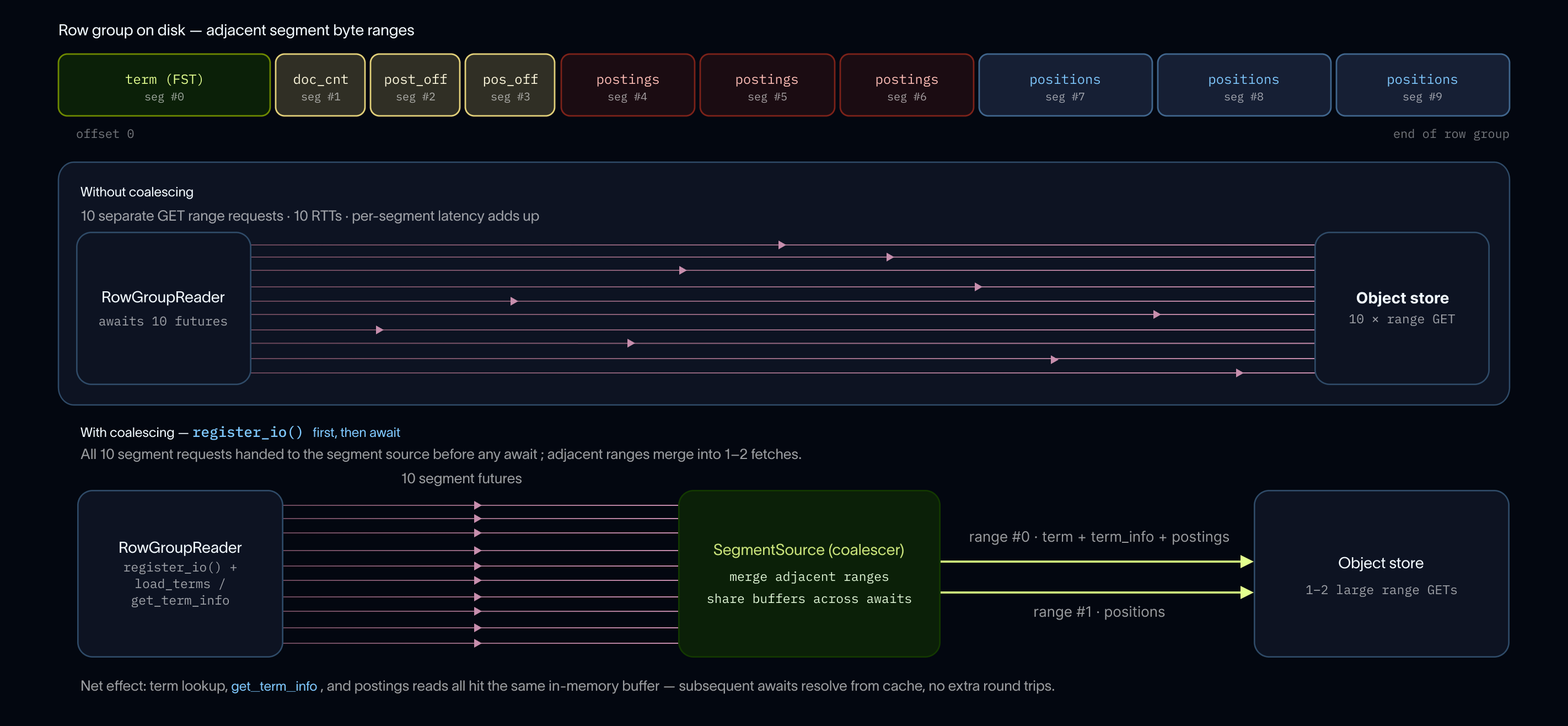
Our earlier blog post outlined how we organize our inverted index data into row-groups. Each row-group read has two phases: range registration, then decode. The reader resolves the term against the FST, reads its term_info entry to obtain postings (for phrase queries, positions as well) offsets and lengths, and registers all required ranges with the Vortex segment scheduler before issuing any object-store request. The scheduler merges adjacent ranges, combines non-adjacent ranges separated by gaps of up to 1 MB, and caps the coalesced window at 16 MB.
On object storage, each GET carries fixed per-request latency and cost that dominate for small reads, so the number of requests matters. Coalescing trades a little wasted transfer (the sub-1 MB gaps) for fewer round trips, and it's effective here because the layout keeps a term's ranges physically close: row groups are bounded by a 32 MB postings budget, and postings and positions flush in ~2 MB chunks aligned on shared document boundaries. A phrase lookup against a selective term resolves to one GET covering term_info, postings, and positions; a non-phrase lookup resolves to one GET covering term_info and postings. A single GET is bounded above by the row-group budget regardless of term frequency.
Once a row group's ranges are fetched, decode happens entirely within the returned buffer, with no further object-store requests. Even seeking is local: block-bitpacked deltas record their per-block bit width inline, so skipping a block advances the cursor by a constant offset without decoding it and without issuing a GET. So the only object-store requests a query makes are the per-row-group reads themselves. Query latency is therefore bounded by the number of row groups surviving pruning, with each GET bounded by the row-group byte budget. The 100 ms round trip enters the latency budget exactly that many times.
Three query shapes, three lookup paths
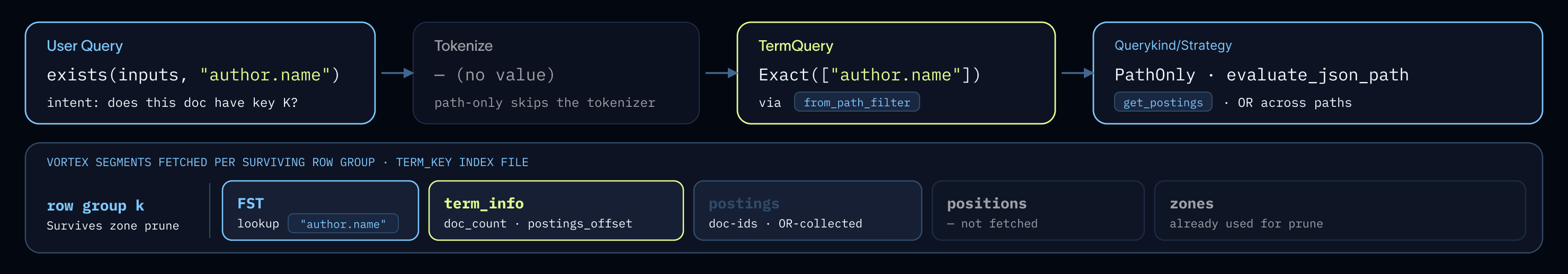
Once routing has handed the predicate to the index layout, each of the three query shapes maps directly onto the v2 columns (term, term_info, postings, positions).
Path-only (json_key) walks the term_key FST and returns postings. Positions are never read since this isn’t a phrase query. The decoded postings become a row-index mask the parent layout reader uses for filtering. This is the cheapest of the three shapes and the one zone-level pruning helps most: a prefix-pattern path query (json_key(inputs, "author.%")) typically skips most row groups before any FST work happens (our FSTs are partitioned).
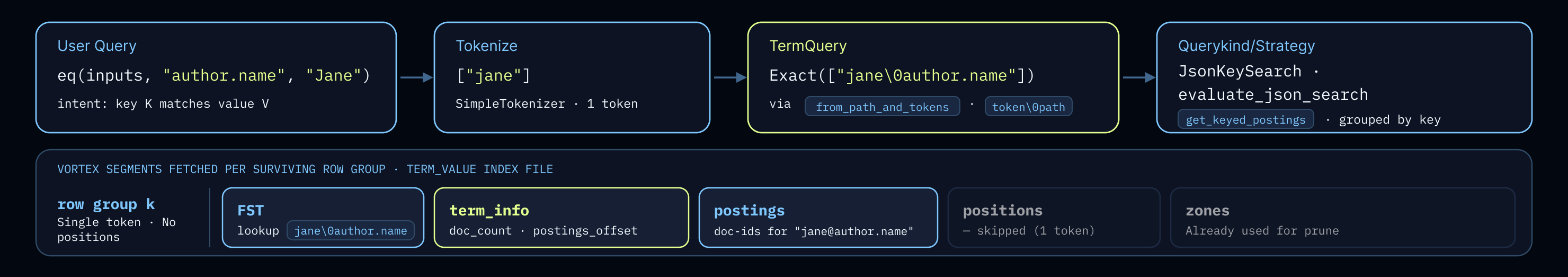
Keyed-search (json_key_search) does one or more FST lookups against term_value, using the token\\0path keying introduced in the v2 layout. A single-token lookup is a single FST exact-match plus a single postings fetch. Multi-token phrase variants intersect postings first, then fall through to PhraseQuery for adjacency.
Full-text (search) reuses the same term_value FST in two modes. For plain-text columns it's an exact lookup. For free-text over JSON values, the token\\0 prefix scan walks every path the token appears under and unions their postings: one FST serving both keyed and unkeyed search, no second dictionary, no extra IO.
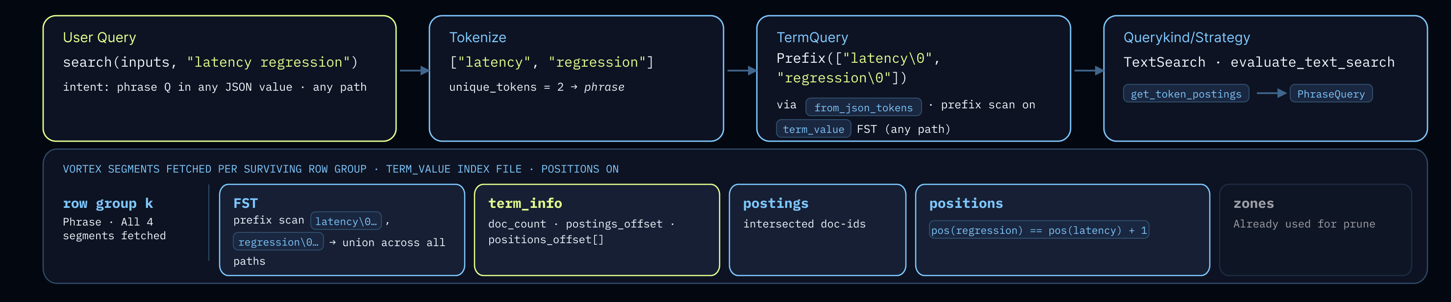
Multi-token phrases on any of the three shapes run through PhraseQuery, which works in two stages: first intersect postings to narrow the candidate documents, then decode positions only for those candidates and verify adjacency. Because position decode is gated behind the postings intersection, a phrase query that matches few documents pays almost no positions IO. That asymmetry is exactly what the separate positions column was designed to enable.
Handling recently ingested data
Observability queries skew hard toward recent data, and customers expect a trace they just ingested to be searchable within seconds for debugging. The "indexes built inline during ingestion" construction model from the previous section is what makes that possible, but it requires the read path to span two storage tiers:
- L0: local SSD on the ingestion node. When ingestion accepts a batch of runs to ingest, the per-column inverted index for that batch is written to local SSD, not durably to object storage. Latency from "trace committed" to "L0 index visible" is therefore very fast.
- L1: object storage. A best-effort compaction in the ingestion service promotes L0 segments and their indexes to object storage; anything ingestion doesn't get to is picked up by the dedicated compaction service, including reconstructing indexes where necessary.
Routing at query time keeps the two tiers coherent without coordination. Our cluster manager already does sticky routing: queries for a given tenant and tracing project go to the node that most recently wrote for that scope. So leading-edge queries land on the writer node, where the layout reader composes that node's in-memory L0 indexes alongside the L1 indexes for older segments. It's the same LayoutReader tree as everywhere else, just with some children pointing at local SSD instead of object storage. A query spanning the last hour transparently mixes L0 reads on the writer node with L1 reads on object storage, and neither the SQL surface nor the predicate routing changes.
There's no separate "live tail" mode and no eventually-consistent gap. Sub-second freshness results from treating L0 as one more tier of the same index, rather than building a parallel system to serve it.
What’s next
We’ll be making and documenting quite a few optimizations to our full text search and inverted index implementation in the near future. Additionally, we’ll be writing more blog posts on SmithDB internals including how we support sub-second stats on massive datasets through a combination of storage layout optimizations and distributed query execution.
//
We’re building SmithDB to solve the systems problems that come with agent observability. If that kind of infrastructure work sounds interesting, we’re hiring.